Model families

Models

Choose among 22 causal and probabilistic model families by the question you need to ask, the assumptions you can defend, and the operations the model actually supports.

Explore 27 maintained examples visually, then use an SDK in software or review agent integration for authorized model requests.

Models in practice

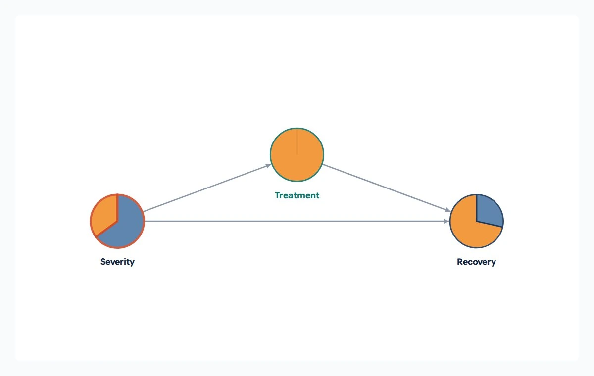
Severity points to Treatment and Recovery; Treatment also points to Recovery. Each circular node contains colored probability slices. — Treatment Effect with Severity Confounding
Bayesian belief network (BBN)
Separate what you observed from what could change under a decision, so a treatment, policy, or operational choice is not mistaken for a correlation.
A network of uncertain variables that updates their probabilities when you learn something new. This example separates a treatment's apparent association with recovery from its effect under stated causal assumptions.
Does recovery differ because of treatment, or because the treated patients started out sicker?
The circles are variables; their slices show probabilities of the possible states. Arrows encode this example's assumptions: severity matters for both treatment assignment and recovery. Treatment is fixed to treated in the pictured scenario.
Synthetic example, not real patient, customer or operational data.
Discrete Bayesian networks Explore this example Software development kit (SDK) guide
Variables and symbols
Severity
How ill the patient is before treatment: mild or severe.
Treatment
Whether the patient is in the control or treated group.
Recovery
Whether recovery occurs: no or yes.

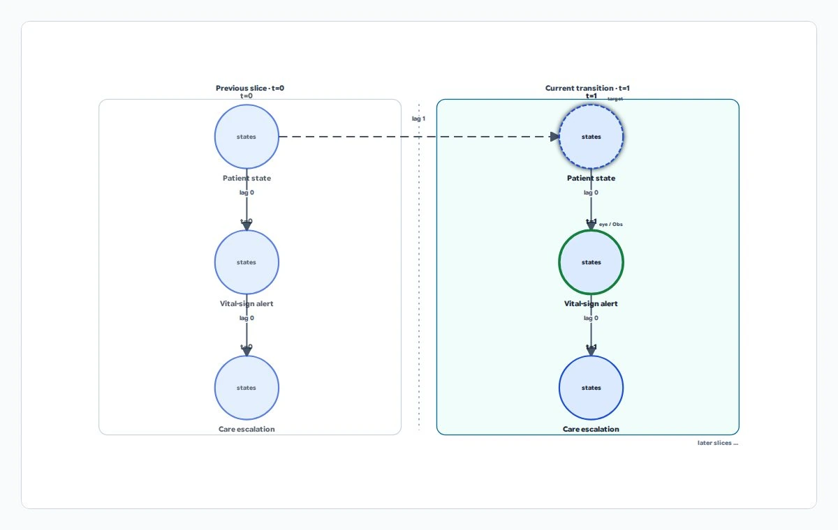
Two time panels repeat Patient state, Vital-sign alert and Care escalation. A dashed arrow links patient state across rounds. — Early Warning for Patient Deterioration
Dynamic Bayesian network (DBN)
Turn a stream of noisy alerts into an updated state estimate and test how a modeled action changes later risk.
A Bayesian network repeated over time. It relates today's uncertain state to the next one, so a new observation can update your estimate of what is happening.
What does an abnormal vital-sign alert tell us about the patient's current condition?
The two panels are successive ward rounds, not two patients. Solid arrows connect variables within a round; the dashed arrow carries patient state into the next round. The highlighted alert is entered evidence, not a diagnosis.
Synthetic example, not real patient, customer or operational data.
Discrete dynamic Bayesian networks Explore this example Software development kit (SDK) guide
Variables and symbols
Patient state
The modeled condition: stable, deteriorating or critical.
Vital-sign alert
The observed warning signal: normal or abnormal.
Care escalation
The care category: routine or escalated.
t, lag, Obs
t is the round index. Lag 0 means the same round; lag 1 means the next. Obs means observation.

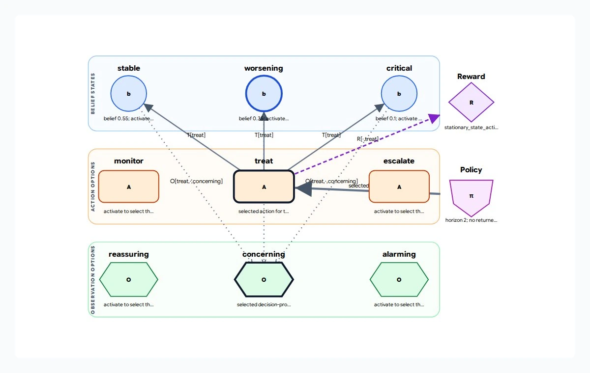
Three rows show stable, worsening and critical states; monitor, treat and escalate actions; and reassuring, concerning and alarming observations, with reward and policy symbols beside them. — Adaptive Care under Partial Observation
Partially observable Markov decision process (POMDP)
Compare action policies when the system’s true state cannot be observed directly.
A model for choosing a sequence of actions when the true situation is only partly known. It tracks beliefs about that situation and weighs possible actions and their outcomes.
How should a care plan change when a noisy observation is concerning?
Circles are possible patient states, rectangles are actions, and hexagons are observations. The selected treat action and concerning observation illustrate the setup; this screenshot does not show a solved policy or a treatment recommendation.
Synthetic example, not real patient, customer or operational data.
Partially observable decision processes Explore this example Software development kit (SDK) guide
Variables and symbols
State and b
Stable, worsening or critical; b is the belief, or probability assigned to each state.
A and O
A is an action: monitor, treat or escalate. O is an observation: reassuring, concerning or alarming.
T and R
T describes state changes after an action. R is the reward score assigned to outcomes and actions.
Policy (pi)
The rule for selecting actions. Horizon 2 means planning over two decision steps.

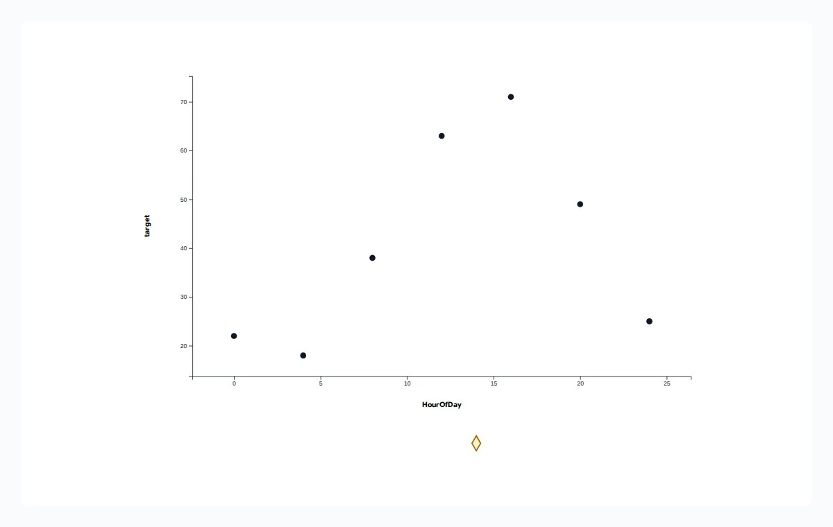
Seven observed demand points on a chart with HourOfDay horizontally and target vertically; a prediction-input diamond sits below the chart. No forecast curve is displayed. — Hospital Demand Forecast
Gaussian process (GP)
Estimate an unmeasured point and see how uncertainty grows away from observed data.
A model that learns how a numeric quantity varies with its inputs while keeping track of uncertainty. Here the input is time of day and the quantity is emergency arrivals.
How many arrivals might the hospital expect at a time between its observations?
This is a data chart, not a node-and-arrow network: each dot pairs an hour with an observed arrival count. It shows the seven training observations, not a computed forecast curve or uncertainty interval. The outlined diamond marks the prediction input, not an arrival count.
Synthetic example, not real patient, customer or operational data.
Gaussian processes Explore this example Software development kit (SDK) guide
Variables and symbols
HourOfDay
The horizontal input: hours from 0 to 24 in this synthetic daily example.
target
The vertical quantity to predict: the example's emergency-arrival count at each observation time.
Prediction input
The requested time is hour 14. A prediction query returns an estimated value and its uncertainty separately.

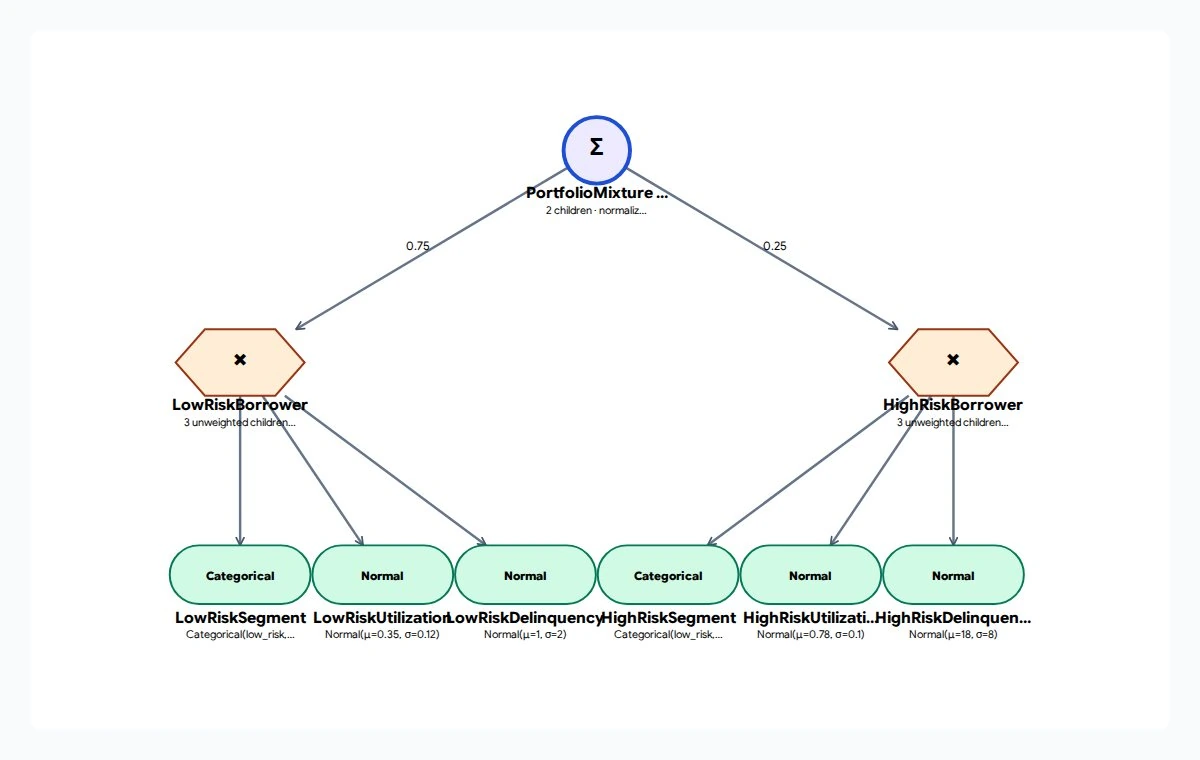
A portfolio sum branches to low-risk and high-risk borrower products, each connected to segment, utilization and delinquency distribution leaves. — Borrower Segment Circuit
Probabilistic circuit (PC)
Reuse a structured probability calculation for repeated scoring and marginal queries.
A probability model built from small distributions combined by sums and products. This example mixes two borrower groups with different credit-use and late-payment patterns.
How well does a borrower's credit use and payment history fit the modeled portfolio?
The top sum blends low-risk and high-risk branches with weights 0.75 and 0.25. Product nodes combine the three characteristics within each branch. The leaves describe distributions; these connections are calculation steps, not causal arrows.
Synthetic example, not real patient, customer or operational data.
Probabilistic circuits Explore this example Software development kit (SDK) guide
Variables and symbols
BorrowerSegment
The modeled group: low_risk or high_risk, represented by the Segment leaves.
CreditUtilization
The fraction of available credit used, represented by the Utilization leaves.
DelinquencyDays
Days late on payment, approximated by the Delinquency leaves' normal distributions.
Sum, product, mu, sigma
Sum mixes branches; product combines their inputs. Mu is a normal distribution's mean; sigma is its standard deviation, a measure of spread.

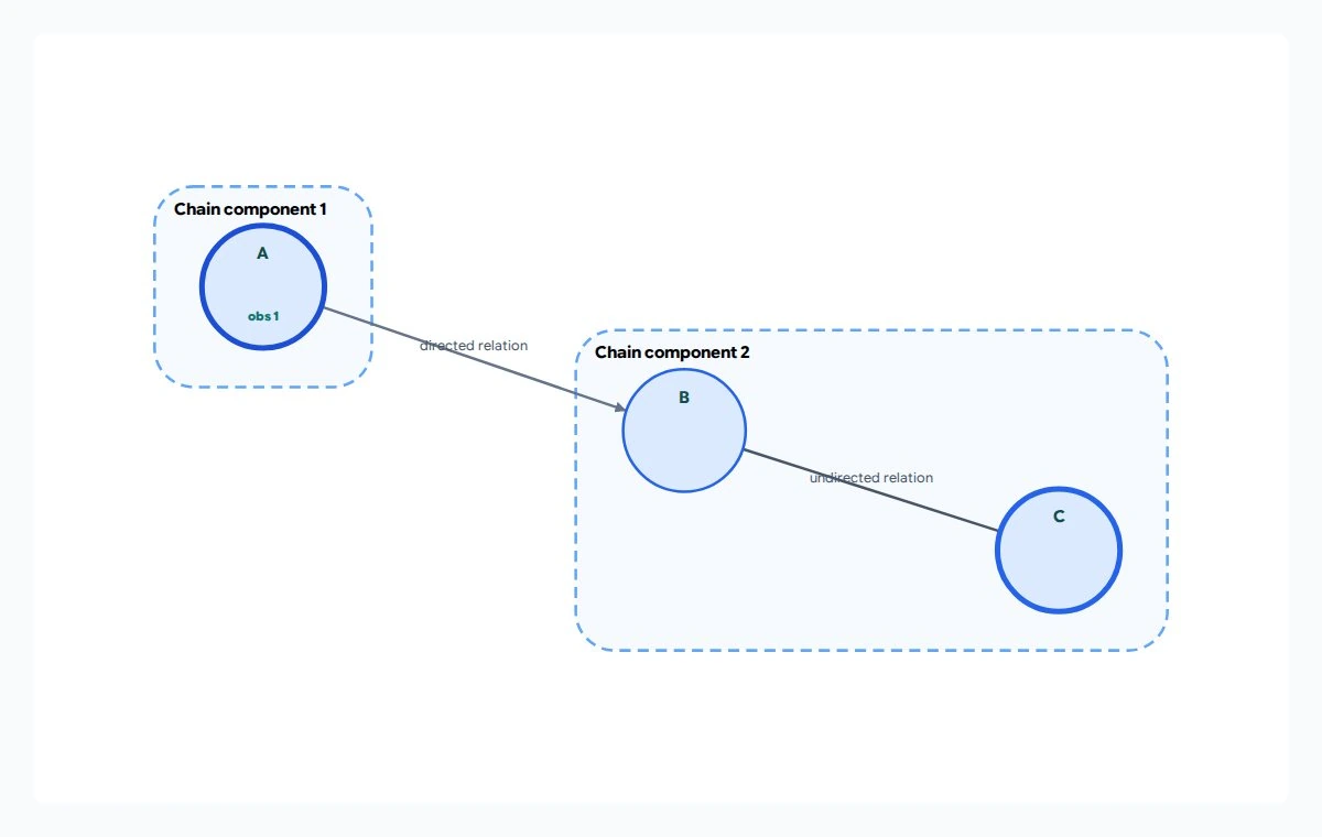
A is alone in chain component 1 and points to B in component 2, where B is joined to C by an undirected line. A is observed in state 1. — Coordinated Service Reliability
Lauritzen-Wermuth-Frydenberg (LWF) chain graph
Calculate risk when one system contains both ordered dependencies and groups of mutually associated variables.
A probability network that groups linked variables into blocks, called chain components. It combines undirected relationships inside a block with directed relationships between blocks, using the LWF probability rules.
How does observing an upstream condition change expectations for a linked pair of service indicators?
A points to B, while B and C share a line without an arrow. The dashed outlines group A separately from the coupled pair B and C. This is an association model, not proof of cause and effect. LWF and AMP chain graphs use different independence rules even when their edge shapes match.
Synthetic example, not real patient, customer or operational data.
LWF chain graphs Explore this example Software development kit (SDK) guide
Variables and symbols
A
The upstream operating-condition indicator in this example; its two states are labeled 0 and 1.
B and C
The two coupled service indicators, each with states 0 and 1. The fixture does not assign names or good/bad meanings to these states.
obs 1
Observation: A has been fixed to state 1 for the probability question.
AMP
Andersson-Madigan-Perlman, a different chain-graph interpretation, not another name for LWF.

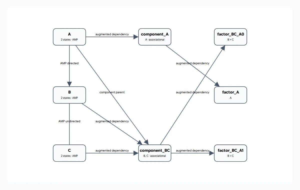
A points to B, B connects without an arrow to C, and auxiliary component and factor boxes show the AMP probability calculation structure. — Finite Discrete AMP Chain Graph
Andersson-Madigan-Perlman (AMP) chain graph
Evaluate dependencies in a mixed-edge system without substituting a different chain-graph interpretation.
A probability network with both directed and undirected links. AMP specifies which variables can be treated as independent once other information is known; these rules differ from those of LWF chain graphs.
How do A's two possible states enter the probability calculation for B and C?
The left-hand A, B and C boxes are the variables. The other boxes show their groups and probability tables, not extra measurements. The augmented-dependency links expose that calculation structure. Directed edges here describe association, not causal effects.
Synthetic example, not real patient, customer or operational data.
AMP chain graphs Explore this example Software development kit (SDK) guide
Variables and symbols
A, B and C
Three abstract variables with states 0 and 1. This mathematical fixture assigns them no real-world units or meanings.
component_A, component_BC
The groups containing A alone and B with C. A is the parent of the second group.
factor_A, factor_BC_A0, factor_BC_A1
Probability tables for A and for the B/C pair when A is 0 or 1. B x C means combinations of B and C states.
LWF
Lauritzen-Wermuth-Frydenberg, the other chain-graph interpretation. Similar-looking graphs are not interchangeable models.

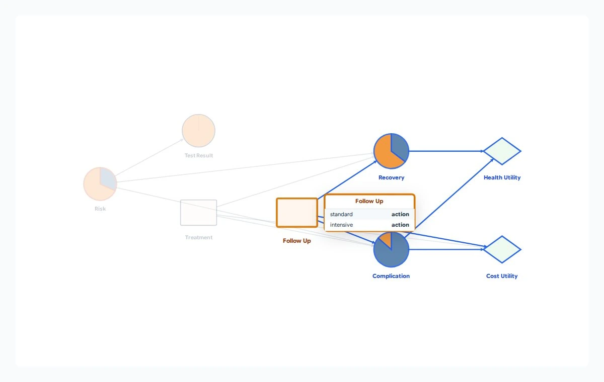
A staged care diagram with Risk, Test Result, Treatment, Follow Up, Recovery, Complication, Health Utility and Cost Utility; Follow Up is highlighted. — Staged Care Pathway Decisions
Influence diagram (ID)
Separate what you observed from what could change under a decision, so a treatment, policy, or operational choice is not mistaken for a correlation.
A probability network extended with choices and scores for their consequences. It represents what is uncertain, what can be decided, and what outcomes are valued.
Which treatment and follow-up choices balance recovery, complications and cost under the model's assumptions?
Circles represent uncertain events, rectangles represent decisions, and diamonds represent utility scores. The highlighted follow-up stage shows its available choices and downstream outcomes, not a recommended care plan.
Synthetic example, not real patient, customer or operational data.
Explore this example Software development kit (SDK) guide
Variables and symbols
Risk and Test Result
Baseline risk is low or high; the diagnostic result is negative or positive.
Treatment and Follow Up
Decisions to monitor or treat, and to provide standard or intensive follow-up.
Recovery and Complication
Outcomes: poor or good recovery, and no or serious complication.
Health Utility and Cost Utility
Model-defined scores for health outcomes and cost. Utility is a preference score, not a probability.

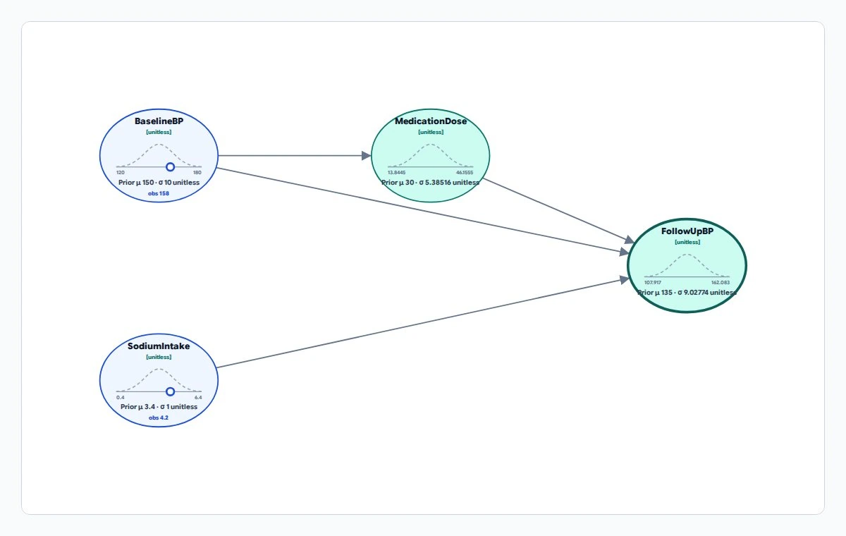
BaselineBP, SodiumIntake and MedicationDose feed FollowUpBP; the numeric nodes show bell-shaped uncertainty curves and entered observations. — Hypertension Treatment Pathway
Linear Gaussian model
Put a numerical range around a forecast, then compare how that range moves under a modeled change.
A model for numeric measurements related by linear equations with bell-shaped, or Gaussian, uncertainty. This example describes assumptions about blood pressure and treatment.
How does expected follow-up blood pressure change under a different medication dose?
Ovals represent numeric variables; the small curves describe their uncertainty. Arrows show the assumed relationships. The display labels the example's values unitless, so the numbers must not be read as clinical doses or thresholds.
Synthetic example, not real patient, customer or operational data.
Linear Gaussian models Explore this example Software development kit (SDK) guide
Variables and symbols
BaselineBP and FollowUpBP
BP means blood pressure: the starting systolic pressure and the pressure at follow-up.
SodiumIntake
The modeled amount of sodium consumed.
MedicationDose
The modeled treatment amount. No clinical unit is declared in this fixture.
Prior, mu, sigma, obs
Prior is uncertainty before entered evidence; mu is the mean, sigma the standard deviation (spread), and obs an observation.

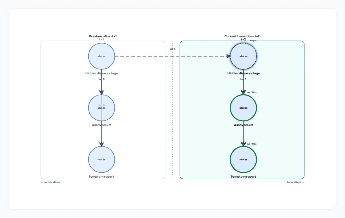
Two visits show Hidden disease stage linked across time with Assay result and Symptom report observation nodes below it. — Hidden Disease Progression from Noisy Tests
Hidden Markov model (HMM)
Turn a stream of noisy alerts into an updated state estimate and test how a modeled action changes later risk.
A time-based probability model whose underlying state cannot be observed directly. Instead, imperfect measurements provide clues about that hidden state.
Which disease stage best explains a sequence of assay results and symptom reports?
Each panel is a visit. The hidden disease state continues between visits and supplies the two observation channels within each visit. Highlighted test and symptom nodes mark entered evidence, not certain knowledge of the disease stage.
Synthetic example, not real patient, customer or operational data.
Explore this example Software development kit (SDK) guide
Variables and symbols
Hidden disease stage
The unobserved category: remission, active or advanced.
Assay result
An imperfect test with a negative or positive result.
Symptom report
An imperfect report of mild or severe symptoms.
t, lag, Obs
t indexes visits; lag 0 is within a visit and lag 1 is between visits. Obs means observation.

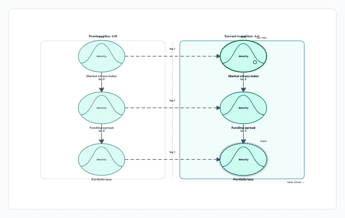
Market stress index, Funding spread and Portfolio loss repeat across two time panels with bell-shaped curves and temporal links. — Liquidity Stress Forecast
Gaussian dynamic Bayesian network (Gaussian DBN)
Keep a continuously changing estimate current as noisy measurements arrive, with uncertainty visible at every step.
A time-based network of numeric quantities with linear relationships and bell-shaped uncertainty. It describes how measurements and their uncertainty evolve together.
How does a market-stress observation change the expected portfolio loss?
The two panels show successive reporting periods. Horizontal dashed arrows carry values between periods; vertical arrows connect quantities in one period. The curves denote numeric uncertainty, not price-history charts.
Synthetic example, not real patient, customer or operational data.
Gaussian dynamic models Explore this example Software development kit (SDK) guide
Variables and symbols
Market stress index
A standardized stress measure in z-score units, or standard deviations from a reference mean.
Funding spread
A borrowing-cost spread in basis points (bps); one basis point is 0.01 percentage point.
Portfolio loss
The modeled loss expressed as a percentage.
t, lag, Obs
t is the reporting period; lag 0 is within a period and lag 1 is between periods. Obs means observation.

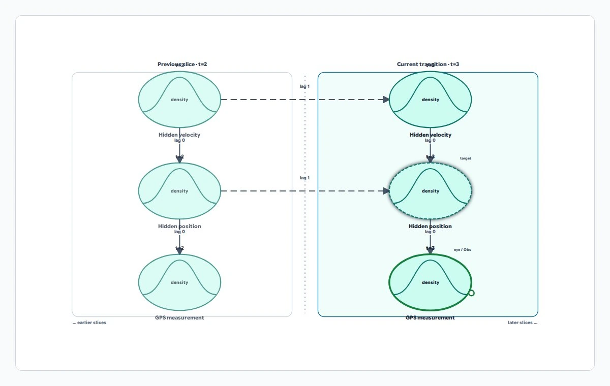
Hidden velocity and Hidden position continue between two time panels, with a GPS measurement node below position in each panel. — Vehicle Position from Noisy Sensors
Kalman state-space model
Keep a continuously changing estimate current as noisy measurements arrive, with uncertainty visible at every step.
A linear model that separates a changing hidden state from noisy measurements of it. Kalman filtering combines the motion assumptions and incoming measurements to estimate that state.
Where is the vehicle likely to be when its position sensor is noisy?
Two time panels distinguish hidden velocity and position from the observed sensor reading. Curves represent Gaussian, or bell-shaped, uncertainty. A highlighted measurement is input evidence, while the marked position node is the estimation target.
Synthetic example, not real patient, customer or operational data.
Explore this example Software development kit (SDK) guide
Variables and symbols
Hidden velocity
The vehicle's unobserved velocity in meters per second (m/s).
Hidden position
The vehicle's unobserved position in meters (m).
GPS measurement
A noisy position reading from the Global Positioning System (GPS), in meters.
t, lag, Obs
t indexes time steps; lag 0 is within a step and lag 1 is between steps. Obs means observation.

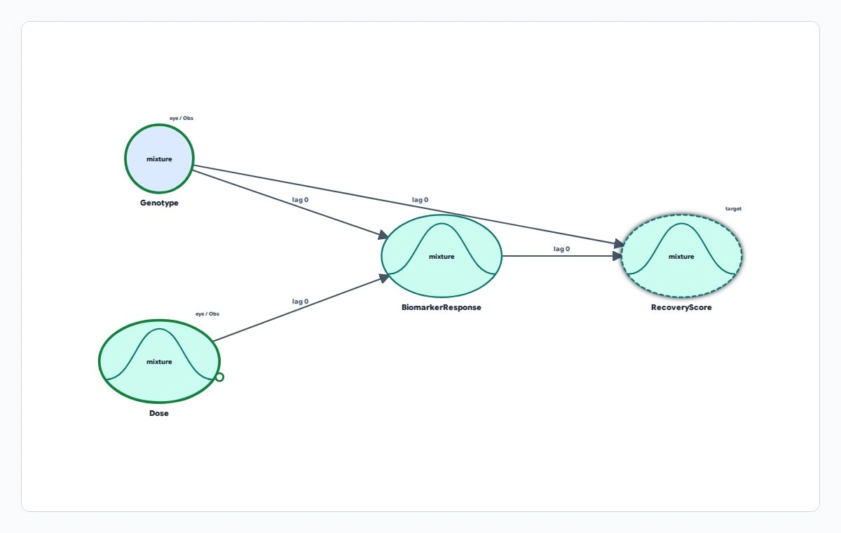
Genotype and Dose point to BiomarkerResponse, which points to RecoveryScore; Genotype also connects directly to RecoveryScore. — Genotype-Aware Treatment Response
Conditional linear Gaussian (CLG) model
Compare numerical outcomes without pretending that every category follows the same response curve.
A model combining categories and numeric quantities. Each category selects a linear relationship with Gaussian, or bell-shaped, uncertainty for the numeric part.
How does the expected response to a dose differ between genotype categories?
The genotype circle is categorical; the curved ovals are numeric. Together genotype and dose inform biomarker response, which informs recovery. Mixture means combining category-specific numeric distributions, not mixing treatments.
Synthetic example, not real patient, customer or operational data.
Conditional linear Gaussian models Explore this example Software development kit (SDK) guide
Variables and symbols
Genotype
The categorical genetic response group, including the observed variant state.
Dose
The modeled treatment amount.
BiomarkerResponse
A numeric change in the biological marker used by this example.
RecoveryScore
A numeric outcome score. These example quantities do not establish clinical scales or thresholds.
Obs and lag 0
Obs means observation; lag 0 indicates a relationship within the same modeled moment.

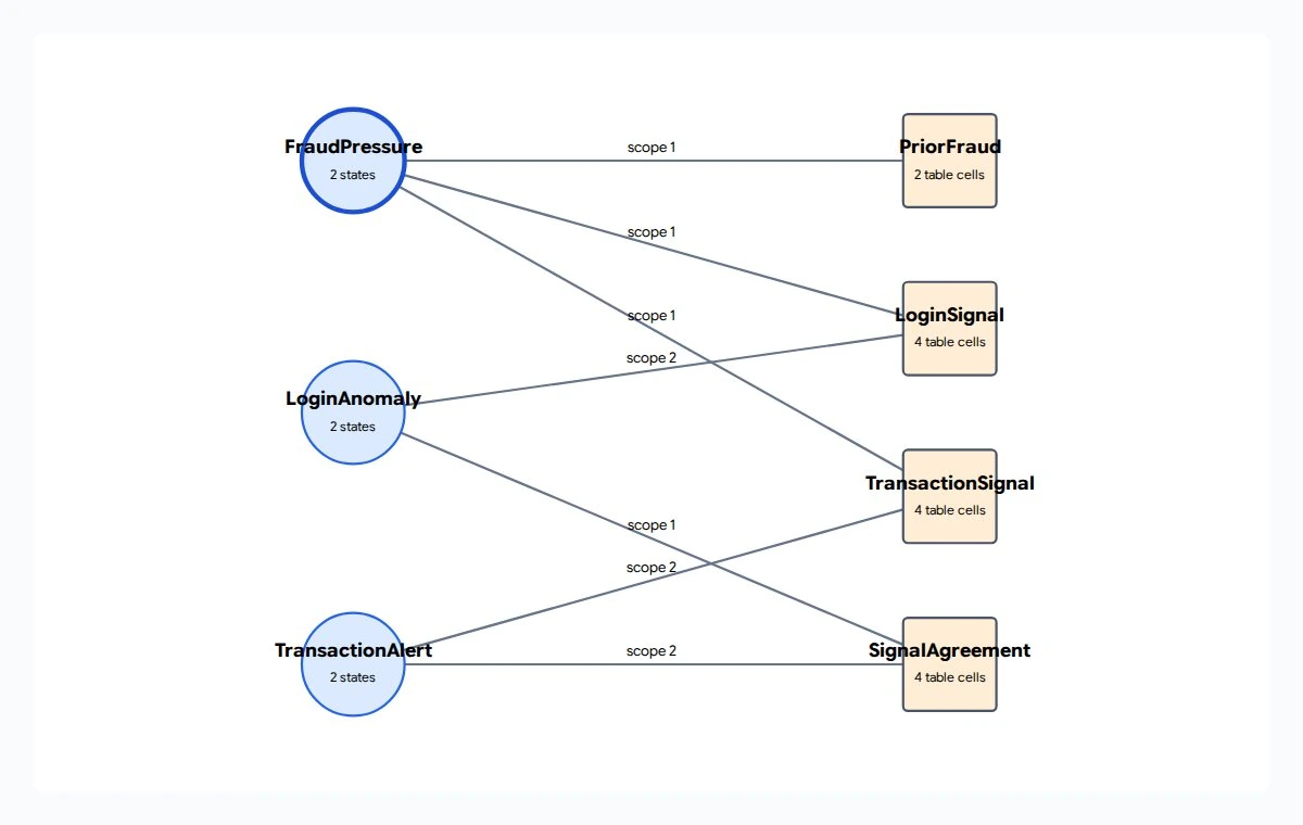
FraudPressure, LoginAnomaly and TransactionAlert circles connect to PriorFraud, LoginSignal, TransactionSignal and SignalAgreement factor squares. — Coordinated Fraud Signals
Factor graph
Combine overlapping constraints into one inspectable probability calculation without forcing an artificial direction on every relationship.
A probability model that separates variables from factors: tables scoring combinations of their possible values. Several factors can connect overlapping groups of variables.
What does a transaction alert imply about fraud pressure when login signals are also related?
Circles are variables and squares are factor tables. Lines identify which variables a factor uses, not causal directions. Scope labels indicate positions within a factor's inputs.
Synthetic example, not real patient, customer or operational data.
Factor graphs Explore this example Software development kit (SDK) guide
Variables and symbols
FraudPressure
The modeled fraud category: low or high.
LoginAnomaly and TransactionAlert
Two signals, each absent or present.
PriorFraud
The factor scoring fraud pressure before the other signals.
LoginSignal, TransactionSignal, SignalAgreement
Factors linking fraud to each signal and linking the two signals to one another. Table cells store combination weights.

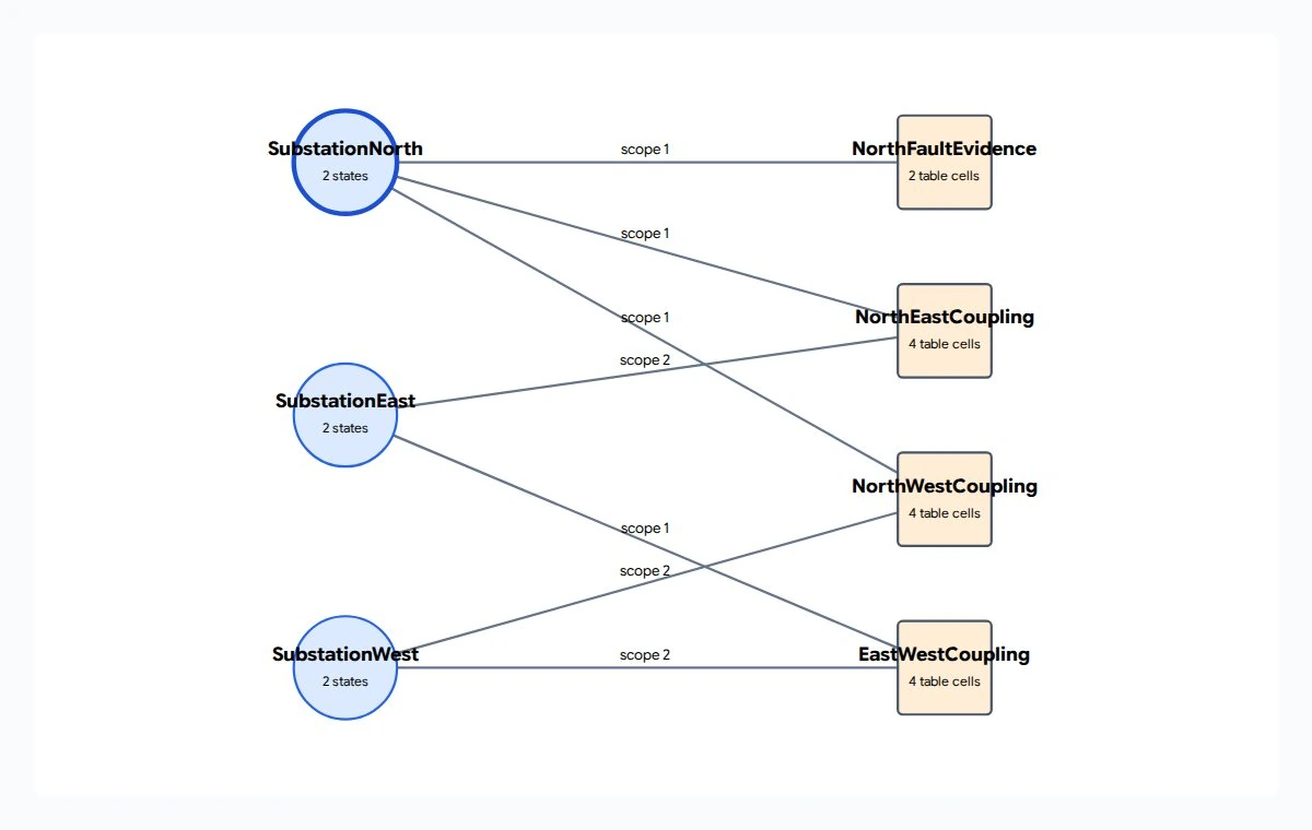
Three substation circles connect to one local evidence factor and three pairwise coupling factors. — Neighborhood Power-Outage Field
Markov random field (MRF)
Combine overlapping constraints into one inspectable probability calculation without forcing an artificial direction on every relationship.
An undirected probability model for mutually related variables. It can describe neighboring sites whose conditions tend to agree, without declaring which one causes another.
What does an outage at one substation imply about the others?
This field is displayed as variables and factor tables. Circles are substations; squares score individual or paired conditions. Coupling means a statistical relationship, not an electrical wiring diagram.
Synthetic example, not real patient, customer or operational data.
Explore this example Software development kit (SDK) guide
Variables and symbols
SubstationNorth, SubstationEast, SubstationWest
The three sites, each in the normal or outage state.
NorthFaultEvidence
The factor scoring the northern substation's condition.
NorthEastCoupling, NorthWestCoupling, EastWestCoupling
Tables scoring how each pair's conditions fit together. Scope identifies a factor's variable inputs.

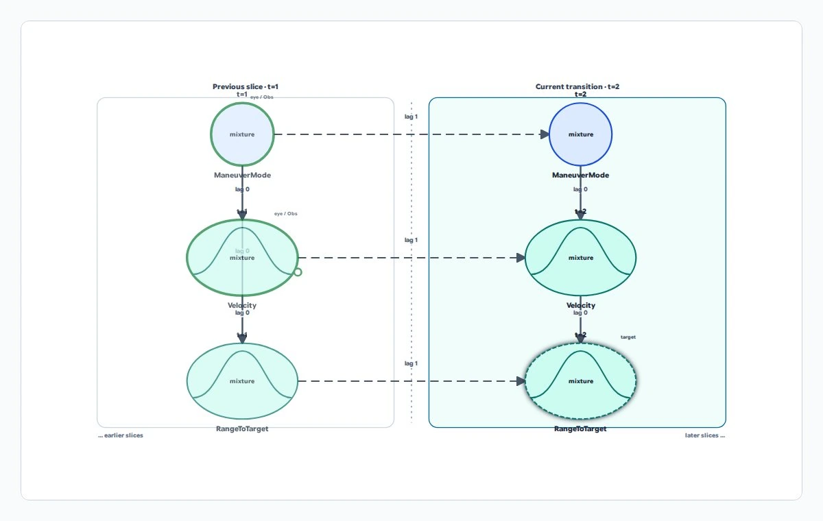
ManeuverMode, Velocity and RangeToTarget appear in two time panels with within-step and cross-step arrows. — Maneuvering Aircraft Tracker
Conditional linear Gaussian dynamic Bayesian network (CLG DBN)
Track a changing numerical system even when its behavior switches between distinct operating modes.
A time-based model combining discrete modes with numeric measurements. The mode selects a linear, Gaussian motion pattern as the system evolves.
How does an evasive maneuver change the expected range to the tracked aircraft?
Two time panels repeat the maneuver category, velocity and range. Dashed arrows carry state forward; numeric curves summarize uncertainty within the mode mixture. The highlighted nodes mark entered evidence and a query target.
Synthetic example, not real patient, customer or operational data.
Hybrid dynamic models Explore this example Software development kit (SDK) guide
Variables and symbols
ManeuverMode
The flight category: steady or evasive.
Velocity
The modeled numeric velocity.
RangeToTarget
The modeled distance to the tracked target; the fixture does not declare a physical unit.
t, lag, Obs
t is the time-step index; lag 0 is within a step and lag 1 is between steps. Obs means observation.

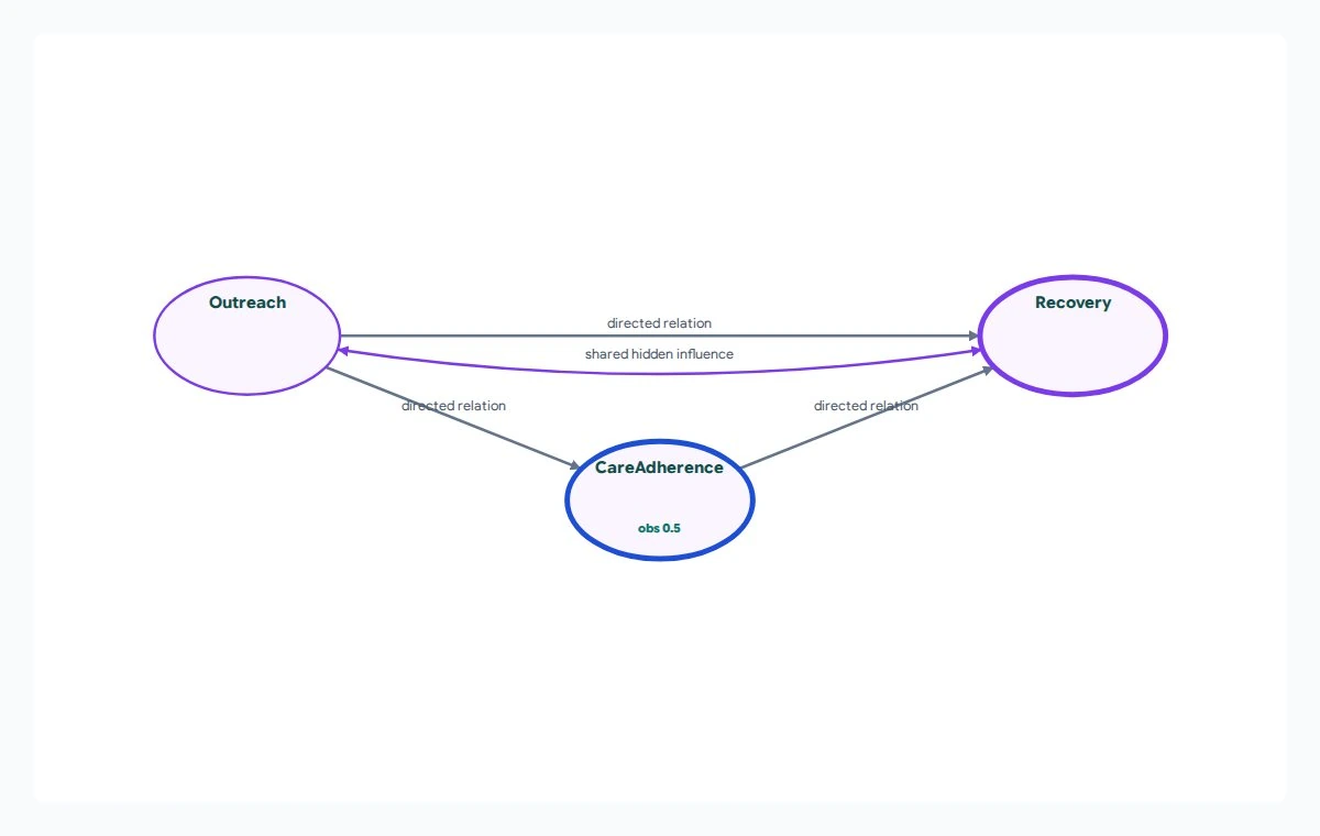
Outreach connects directly to Recovery and through CareAdherence, with an additional curved connection between Outreach and Recovery. — Community Outreach with Hidden Confounding
Latent causal model
Test a decision without silently treating hidden shared causes as if they were measured evidence.
A causal model that allows unmeasured influences to affect more than one observed variable. Latent means hidden; confounding means a shared influence can complicate an apparent cause-and-effect relationship.
How might outreach affect recovery when unmeasured need also influences both?
Directed connections express the example's assumed pathways through outreach and care adherence. The additional curved connection represents shared hidden influence between outreach and recovery. Those assumptions must be justified separately from the picture.
Synthetic example, not real patient, customer or operational data.
Latent causal models Explore this example Software development kit (SDK) guide
Variables and symbols
Outreach
The numeric level of outreach in the model.
CareAdherence
The numeric degree of following the care plan; obs 0.5 is entered evidence.
Recovery
The modeled numeric recovery outcome.
Hidden influence
Unmeasured shared variation, illustrated by community need; it is not an extra measured node in this screenshot.

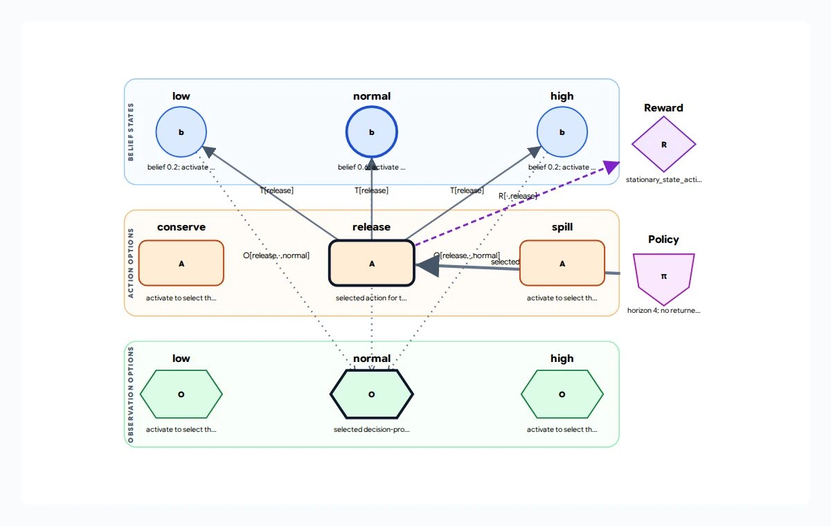
Low, normal and high reservoir states sit above conserve, release and spill actions and matching low, normal and high observations. — Fully Observed Reservoir Operations
Markov decision process (MDP)
Compare action policies when the system’s true state cannot be observed directly.
A model for sequential decisions when each new state is observed exactly. This example is the fully observed special case of a partially observable Markov decision process (POMDP).
Which water-management action best balances future outcomes over four decision steps?
The top row lists possible reservoir states; the middle row lists actions; the bottom row records observations that identify the new state exactly. The pictured release selection is a setup choice, not a returned optimal policy.
Synthetic example, not real patient, customer or operational data.
Explore this example Software development kit (SDK) guide
Variables and symbols
State and b
Reservoir level is low, normal or high; b shows the initial probability assigned to each level.
A and O
A denotes conserve, release or spill actions. O is the exactly observed level after an action.
T and R
T describes level changes after an action. R is the model's reward score.
Policy (pi) and horizon
A policy selects actions; horizon 4 means four decision steps.

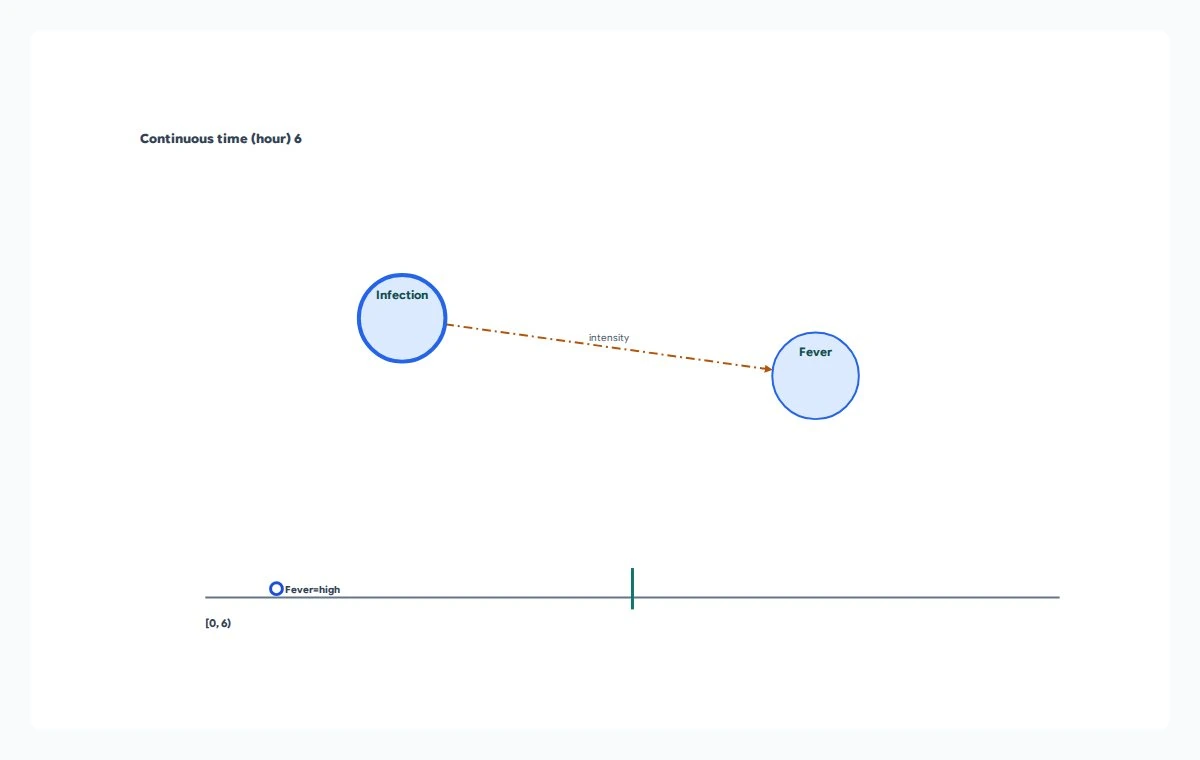
Infection connects to Fever through an intensity link above a continuous-time timeline with a high-fever observation. — Hospital Infection Dynamics
Continuous-time Bayesian network (CTBN)
Estimate state risk between irregular observations instead of forcing events into arbitrary time buckets.
A model of categorical states that can change at any moment, not just at fixed observation times. Rates describe how quickly those changes happen.
What is the modeled infection probability hours after a high-fever observation?
The arrow says the fever transition rates depend on the infection state. The lower timeline marks the entered high-fever observation and the current time cursor; it is not an infection-probability curve.
Synthetic example, not real patient, customer or operational data.
Continuous-time Bayesian networks Explore this example Software development kit (SDK) guide
Variables and symbols
Infection
Whether infection is absent or present.
Fever
Whether fever is normal or high.
Continuous time and intensity
Time is in hours. Intensity means a state-change rate, not symptom severity; the pictured cursor is at hour 6.

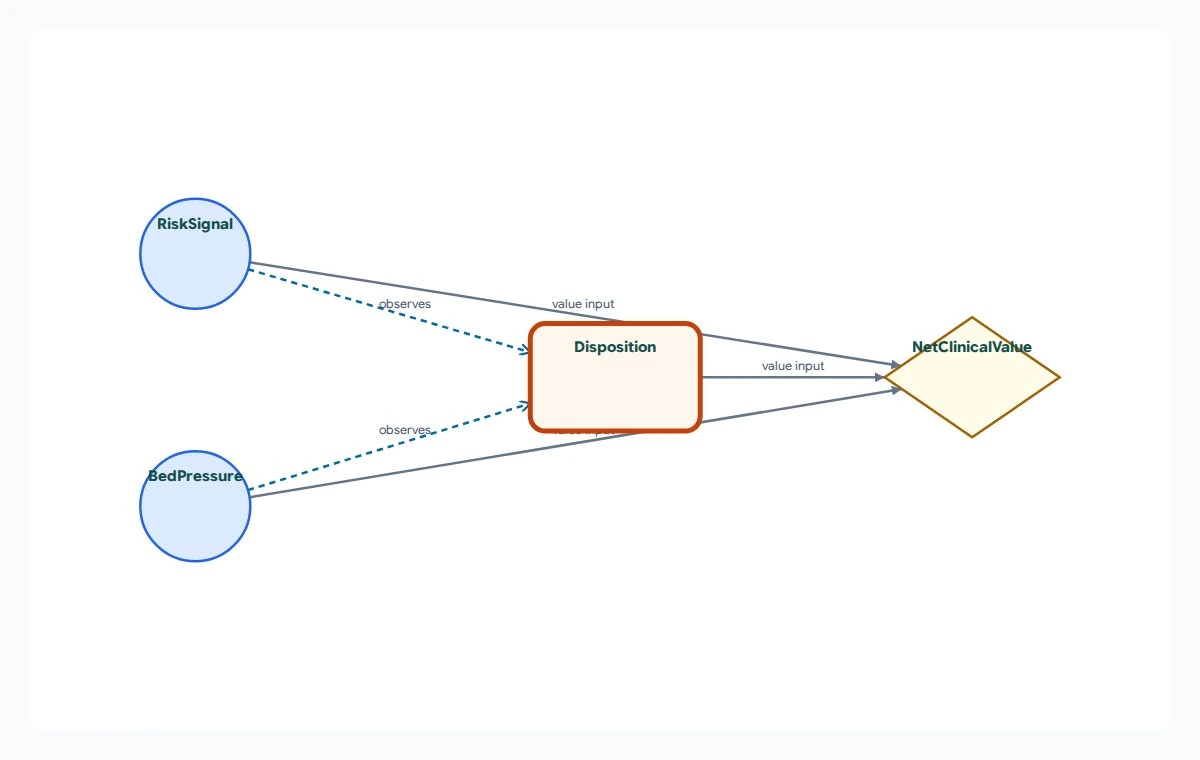
RiskSignal and BedPressure are observed by Disposition; all three connect to NetClinicalValue. — Emergency Department Disposition
Decision analysis network (DAN)
Compare available choices using the information, outcomes, and utility assumptions that were actually declared.
A model relating available information, possible choices and the value of their consequences. It evaluates decisions at the information states that can actually be reached.
How should risk and available beds affect a modeled discharge, observation or admission decision?
Circles are uncertain inputs, the rectangle is a decision, and the diamond is a value score. Dashed arrows mark information available to the decision. No recommended disposition is displayed in this screenshot.
Synthetic example, not real patient, customer or operational data.
Decision analysis networks Explore this example Software development kit (SDK) guide
Variables and symbols
RiskSignal
The observed risk category: low or high.
BedPressure
Capacity is available or constrained.
Disposition
The choice: discharge, observe or admit.
NetClinicalValue
A model-defined score balancing clinical benefit and capacity cost, not a probability or validated clinical rule.

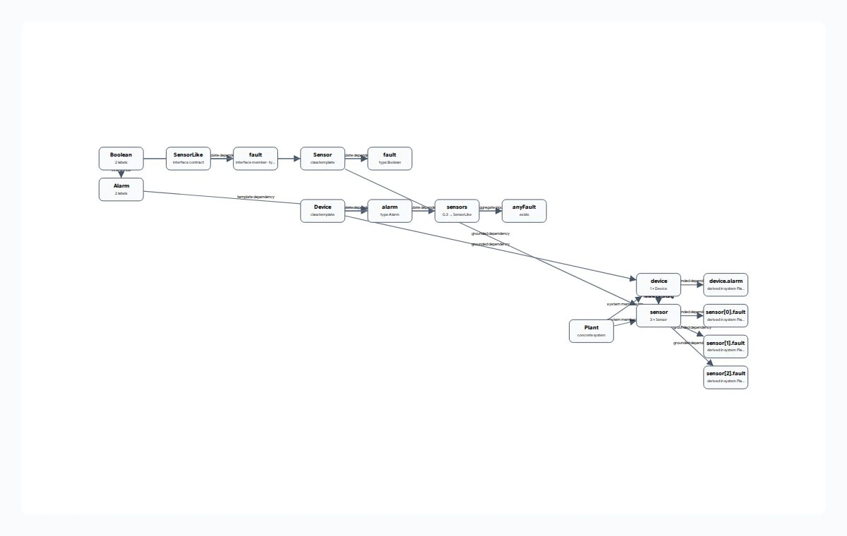
Boolean and Alarm types, a SensorLike interface and Sensor and Device templates connect to Plant instances, device.alarm and three sensor fault attributes. — Finite Discrete PRM / OOBN
Probabilistic relational model (PRM) / object-oriented Bayesian network (OOBN)
Define a repeated probabilistic pattern once, then query individual objects in a finite connected system.
A probability model assembled from reusable object templates and their relationships. The same sensor template can describe several sensors without writing a separate model for each one.
How likely is a device alarm when any of its connected sensors may be faulty?
The upper boxes are types, interfaces and templates; the lower boxes are the concrete Plant, device and three sensor instances. Arrows include template and object dependencies, so not every box is a measured variable.
Synthetic example, not real patient, customer or operational data.
Relational Bayesian models Explore this example Software development kit (SDK) guide
Variables and symbols
sensor[0].fault, sensor[1].fault, sensor[2].fault
Whether each of the three sensors is faulty: false or true.
device.alarm
Whether the device alarm is false or true.
anyFault and sensors
anyFault asks whether at least one connected sensor is faulty; sensors is the device's reference to those objects.
Boolean, Alarm, SensorLike, Sensor, Device, Plant
Boolean and Alarm define value types; SensorLike defines a shared interface; Sensor and Device are reusable templates; Plant is the concrete collection of instances.

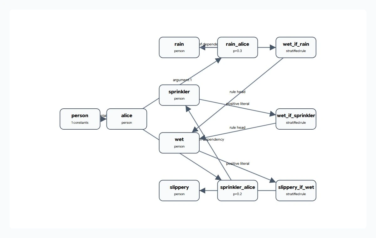
The alice entity connects to rain and sprinkler facts, which feed wet rules and then slippery_if_wet. — Finite Probabilistic Logic Program
Probabilistic logic program (PLP)
Trace a probability through explicit rules so the route from uncertain facts to a conclusion remains inspectable.
A model combining uncertain facts with logical rules. It calculates how uncertainty in the facts affects conclusions obtained by following those rules.
How likely is a slippery condition if either rain or a sprinkler can make things wet?
Boxes show the named entity, fact types, uncertain facts and rules. Rain and sprinkler facts can each imply wet, and wet implies slippery. Rule links express logical dependencies, not an estimated causal effect.
Synthetic example, not real patient, customer or operational data.
Probabilistic logic programs Explore this example Software development kit (SDK) guide
Variables and symbols
person and alice
person is the entity type; alice is the single named example entity, not real personal data.
rain_alice and sprinkler_alice
True/false uncertain facts for that entity, with probabilities p = 0.3 and p = 0.2.
wet and slippery
True/false conclusions derived by the rules.
wet_if_rain, wet_if_sprinkler, slippery_if_wet
The three implication rules. A rule head is its conclusion; a positive literal is an unnegated fact used by a rule.

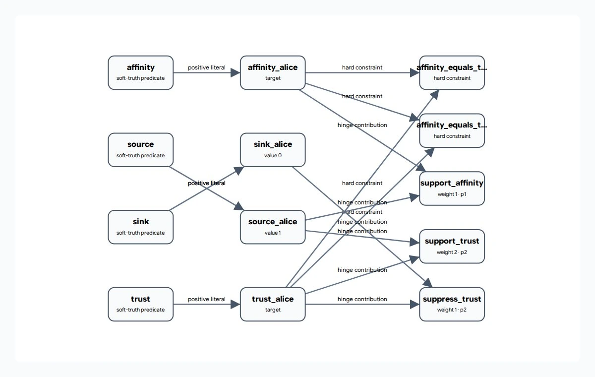
Affinity, source, sink and trust predicates connect to alice values and equality, support and suppression rules. — PSL HL-MRF
Probabilistic soft logic (PSL) / hinge-loss Markov random field (HL-MRF)
Turn conflicting weighted rules into one inspectable soft assignment instead of hiding disagreement behind a binary label.
A model of graded truth values between 0 and 1, constrained by rules. Hard rules must hold; weighted soft rules may be violated at a cost, which the model minimizes.
Which affinity and trust scores best satisfy the supplied rules together?
The diagram connects abstract predicates, their values for alice, and hard or weighted rules. These are soft-truth scores, not calibrated probabilities. Hinge contributions measure rule violations that add to the objective.
Synthetic example, not real patient, customer or operational data.
Probabilistic soft logic Explore this example Software development kit (SDK) guide
Variables and symbols
affinity_alice and trust_alice
Two unknown scores from 0 to 1; these are abstract fixture names, not measured attributes of a real person.
source_alice and sink_alice
Fixed reference scores of 1 and 0 that supply supporting and opposing constraints.
affinity_equals_trust
Two hard rules require the affinity and trust scores to match.
support_affinity, support_trust, suppress_trust
Weighted rules that favor or oppose scores. Weight sets the cost strength; p1 and p2 denote linear and squared violation penalties.

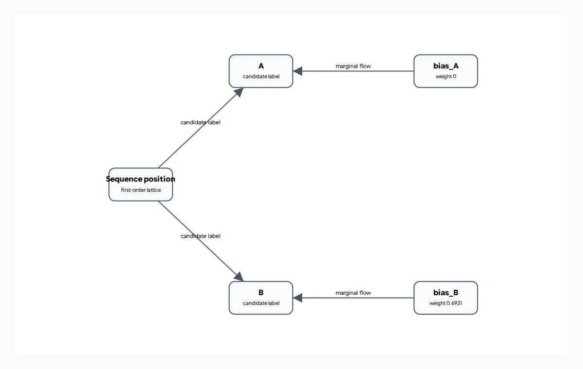
Sequence position branches to candidate labels A and B, connected to bias_A and bias_B feature boxes. — Linear-Chain CRF
Linear-chain conditional random field (CRF)
Label an entire sequence coherently instead of classifying each position without its neighbors.
A model that assigns labels to a sequence while considering observed features and neighboring labels. It models label probabilities given the input sequence.
Which label is most likely at each sequence position under the supplied feature weights?
This small example shows a sequence position, two candidate labels and their bias features. It illustrates the model's labeling structure, not a decoded sentence or a returned label sequence.
Synthetic example, not real patient, customer or operational data.
Linear-chain conditional random fields Explore this example Software development kit (SDK) guide
Variables and symbols
Sequence position
The item in an ordered sequence whose label is unknown.
A and B
The two possible labels. No real-world categories are assigned in this fixture.
bias_A and bias_B
Features scoring each label, with weights 0 and about 0.6931. Weights are scores, not probabilities.

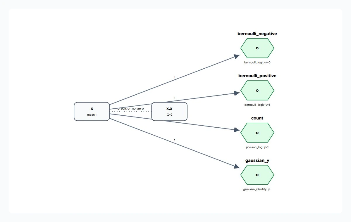
Hidden x connects to a precision entry and four observation nodes: bernoulli_negative, bernoulli_positive, count and gaussian_y. — Sparse Latent-Gaussian GMRF
Sparse latent Gaussian Markov random field (GMRF)
Estimate a large hidden field with local dependence while retaining marginal uncertainty at each location.
A model of hidden numeric quantities with Gaussian uncertainty and a sparse dependence structure. Different types of observations can provide evidence about those hidden quantities.
What does a mix of binary, count and numeric observations imply about the hidden value x?
The rectangle x is the hidden variable. Green observation nodes provide different measurement types. The x,x box is an uncertainty parameter, not another observed variable. This fixture contains only one hidden dimension.
Synthetic example, not real patient, customer or operational data.
Sparse Gaussian Markov random fields Explore this example Software development kit (SDK) guide
Variables and symbols
x
An abstract hidden real-valued quantity with prior mean 1; no physical unit is specified.
x,x and Q
The precision entry Q = 2. For this one-dimensional prior, precision is the inverse of variance, which measures uncertainty.
bernoulli_negative and bernoulli_positive
Binary observations with recorded values 0 and 1, related to x through a logit link.
count and gaussian_y
A count observation of 1 and a numeric observation of 1.2. The latter uses a bell-shaped measurement model. O means observation.

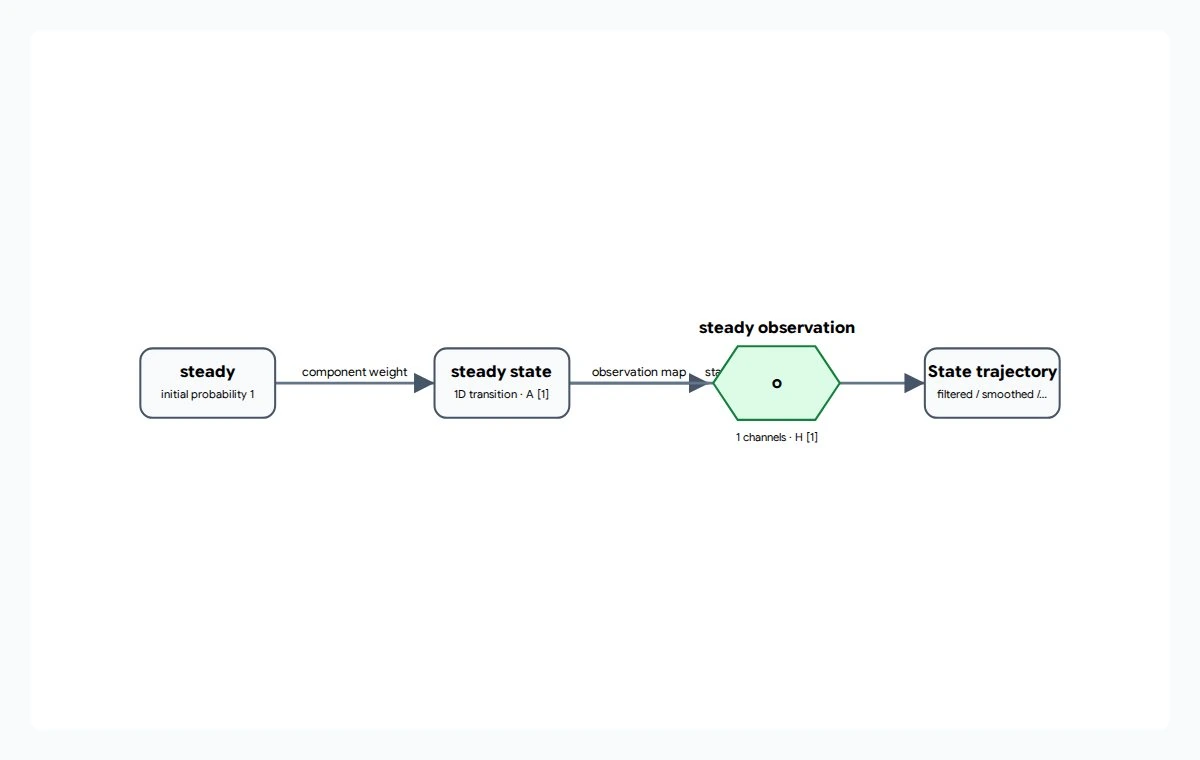
A steady regime connects to steady state, steady observation and a State trajectory output box. — Switching Linear Dynamical System
Switching linear dynamical system (SLDS)
Track a continuous system without assuming it stays in one operating regime.
A time-based numeric model that can switch between distinct linear motion or behavior regimes. Within each regime, it tracks hidden state and noisy observations.
How can a hidden state trajectory be estimated from a sequence of noisy measurements?
The diagram connects a regime, its state dynamics, its measurement model and the trajectory output. This starter has only the steady regime, so it does not demonstrate an actual regime switch or a computed trajectory.
Synthetic example, not real patient, customer or operational data.
Switching linear dynamical systems Explore this example Software development kit (SDK) guide
Variables and symbols
steady
The single regime in this fixture, with initial probability 1.
steady state
One hidden numeric state; 1D means one-dimensional. A is its linear transition coefficient.
steady observation
One noisy measurement channel. H maps hidden state to a predicted measurement; O means observation.
State trajectory
The series of state estimates over time, produced by an analysis rather than displayed here.

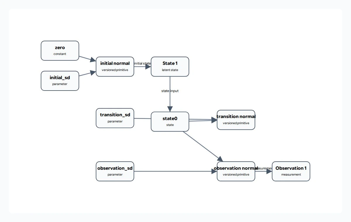
Parameter and expression boxes feed initial normal, transition normal and observation normal distributions, with State 1 and Observation 1 nodes. — Nonlinear Non-Gaussian State-Space Model
Nonlinear, non-Gaussian state-space model
Estimate hidden state when straight-line dynamics and Gaussian noise are not credible assumptions.
A model separating hidden state evolution from observations, with flexible equations and probability distributions. It is not restricted to linear relationships or bell-shaped uncertainty.
How can observations update a hidden state when more flexible dynamics are needed?
The boxes expose the expressions and distributions used for initial state, state transitions and measurements. This particular starter uses normal distributions and simple dynamics; it does not itself demonstrate non-Gaussian behavior.
Synthetic example, not real patient, customer or operational data.
Nonlinear state-space models Explore this example Software development kit (SDK) guide
Variables and symbols
State 1 and state0
The single hidden state and its expression reference; state0 uses zero-based indexing, not a second physical variable.
Observation 1
The single measurement channel for that state.
initial_sd, transition_sd, observation_sd
sd means standard deviation: the spread of initial uncertainty, state-change noise and measurement noise.
zero and normal
zero is the constant 0. Normal means a Gaussian, or bell-shaped, distribution in each of the three depicted mechanisms.